Residual Networks ✅

1 Theoretical background

Let’s look at how to improve the performance of a neural network by adding more layers.

Consider a function that we are learning:

$$f:X\to Y$$ with respect to the training data $\{x_i,y_i\}$.

Traditional wisdom is that we are to build networks with ever increasing number of layers to learn $f$.

$${\mathbf{NN}}_k(x)=L_k\circ L_{k_1}\circ L_{k-2}\circ \cdots \circ L_2\circ L_1(x)$$

We can see the learned network ${\mathbf{NN}}_k$ as a function that is some distance away from $f$.

image.png

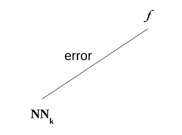
Suppose we wish to improve the approximation an additional layer:

$${\mathbf{NN}}_{k+1}(x)=L\circ {\mathbf{NN}}_k(x)$$

How can we guarantee that ${\mathbf{NN}}_{k+1}$ will be guaranteed to be an improvement over ${\mathbb{NN}}_k$?

If we design $L$ as a residual layer, then we have that guarantee.

2 What is a residual layer?

A residual layer $L$ is a special architecture based on another neural network block. Consider some neural network module $\mathbf{M}(x)$. Typical choice of $\mathbf{M}$ is either based on $\mathbf{MLP}$ or $\mathbf{Conv}\mathbf{2}\mathbf{D}$ depending on the learning task.

The residual layer $L$ is defined as:

$$L(x)=\mathbf{M}(x)+x$$

It is schematics is as follows:

image.png

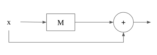
We note that $\mathbf{M}:X\to X$ must preserve the dimensionality of the input since $M(x)+x$ must be a valid operation.

3 Why residual layers help?

Claim:

$M(x)$ can learn the function $\mathbf{zero}(x)=0$ by default. We just need to initialize the weights to 0. Then MLP or Conv2D layer would just produce zero vectors as its output.

Claim:

$L(x)$ can learn the function $\mathbf{id}(x)=x$ by default.

1. By definition $L(x)=M(x)+x$
2. By default $M(x)=0$, thus $L(x)=x$ by default.

Claim:

By default ${\mathbf{NN}}_{k+1}={\mathbf{NN}}_k$.

1. By default $L(x)=x$.
2. Thus, by default ${\mathbf{NN}}_{k+1}(x)=L({\mathbf{NN}}_k(x))={\mathbf{NN}}_k(x)$.

Therefore, we can see that by adding the residual layer, we cannot do worse than the previous network.

4 Building the MLP residual layer.

Let’s build a MLP residual layer.

import torch
import torch.nn as nn
import torch.nn.functional as F
from torch.utils.data import DataLoader, random_split
from torchsummaryX import summary
import numpy as np
import time
from tqdm.notebook import trange, tqdm
import my

device = torch.device('cuda:0' \
                      if torch.cuda.is_available() \
                      else 'cpu')
device

device(type='cuda', index=0)

class Residual_MLP(nn.Module):
    def __init__(self, input_dim, hidden_dim):
        super().__init__()
        self.mlp = nn.Sequential(
            nn.Linear(input_dim, hidden_dim),
            nn.ReLU(),
            nn.Linear(hidden_dim, input_dim)
        )
    def forward(self, x):
        return self.mlp(x) + x

Let’s try out the MLP residual layer in action.

sample = torch.randn(1, 10)
L = Residual_MLP(10, 100)
print("x.shape", sample.shape)
print("L(x).shape", L(sample).shape)

x.shape torch.Size([1, 10])
L(x).shape torch.Size([1, 10])

5 Residual layer in action

Let’s start with a simply classifier.

N1 = nn.Sequential(
    nn.Flatten(),
    nn.LazyLinear(10),
)

def train(model, dataset, epochs):
    optimizer = torch.optim.Adam(model.parameters())
    loss = nn.CrossEntropyLoss()
    dataloader = DataLoader(dataset, batch_size=128, shuffle=True)
    model = model.to(device)
    for epoch in trange(epochs):
        start = time.time()
        for (xs, targets) in tqdm(dataloader):
            xs, targets = xs.to(device), targets.to(device)
            ys = model(xs)
            optimizer.zero_grad()
            l = loss(ys, targets)
            l.backward()
            optimizer.step()
            with torch.no_grad():
                acc = (ys.argmax(axis=1) == targets).sum() / xs.shape[0]
        duration = time.time() - start
        print("[%d] acc = %.2f loss = %.4f in %.2f seconds." % (epoch, acc.item(), l.item(), duration))

train(N1, mnist, 1)

[0] acc = 0.83 loss = 0.4740 in 6.88 seconds.

Now, we can add a residual layer.

N2 = nn.Sequential(
    N1,
    Residual_MLP(10, 5),
)

train(N2, mnist, 1)

[0] acc = 0.94 loss = 0.3469 in 7.61 seconds.

Let’s add one more residual layer.

N3 = nn.Sequential(
    N2,
    Residual_MLP(10, 5),
)
train(N3, mnist, 1)

[0] acc = 0.95 loss = 0.2087 in 7.37 seconds.

N4 = nn.Sequential(
    N3,
    Residual_MLP(10, 5),
)
train(N4, mnist, 1)

[0] acc = 0.96 loss = 0.1728 in 7.72 seconds.

So, we can see that additional layers incrementally improves the network performance at the expense of the memory requirements of larger models.

The added residual layers brings the function closer to the true function $f$.

image.png