Multi-layer Perceptron ✅

import my.matplotlib_theme
import numpy as np
import matplotlib.pyplot as pl

1 Linear Separability of Binary Classification

Consider the training data:

Inputs: \(X = \{x_i\in\mathbb{R}^d\}\)
Labels: \(Y = \{y_i\in\{0,1\}\}\)

We say that \((X, Y)\) is linear-separable if there exists some hyperplane in \(\mathbb{R}^d\) defined by

\(w\in\mathbb{R}^d\)
\(b\in\mathbb{R}\)

such that:

\[\forall i,\ y_i = \mathrm{sign}(w^Tx + b)\]

#
# Linearly separable dataset
#
np.random.seed(1)

ang = -45 * np.pi / 180
M = np.array([
    [1.0, 0.0],
    [0.0, 2.0]
]) @ np.array([
    [np.cos(ang), np.sin(ang)],
    [-np.sin(ang), np.cos(ang)]
])
L = 3
x0 = np.random.randn(1000, 2) @ M + np.array([-L, L])
x1 = np.random.randn(1000, 2) @ M + np.array([L, -L])

figure = pl.figure(figsize=(6,6))
ax = figure.add_subplot(1,1,1)
ax.scatter(x0[:, 0], x0[:, 1], s=1)
ax.scatter(x1[:, 0], x1[:, 1], s=1)

#
# Separation
#
ax.plot([-8, 8], [-8, 8], '--')
ax.set_aspect('equal');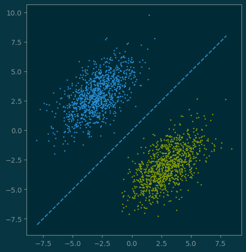

#
# Linearly inseperable dataset
#

import sklearn.datasets

x_donuts, y_donuts = sklearn.datasets.make_circles(1000, noise=0.05, factor=0.5)
x0 = x_donuts[y_donuts == 0]
x1 = x_donuts[y_donuts == 1]

figure = pl.figure(figsize=(6,10))
ax = pl.gca()
ax.scatter(x0[:, 0], x0[:, 1], s=1)
ax.scatter(x1[:, 0], x1[:, 1], s=1)
ax.set_aspect('equal')
ax.set_title('Linearly Inseparable Donuts');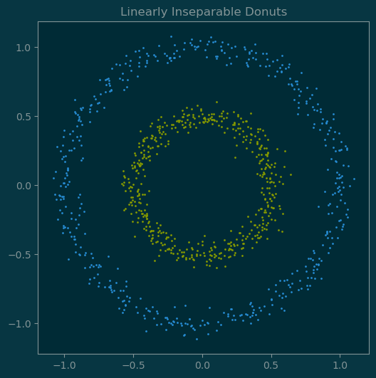

2 Kernel Methods

Suppose \(\{(x_i, y_i)\}\) is not linearly separable. Can we find some transformation \(\phi\) such that \(\{(\phi(x_i), y_i)\}\) becomes linearly separable?

Yes.

The function \(\phi\) is called the kernel.

def kernel(x):
    r = np.linalg.norm(x, axis=-1)
    return np.concatenate([x, r[:, None]], axis=-1)

kernel(x_donuts)[:5].round(3)

array([[ 0.034, -0.575,  0.576],
       [-0.078,  0.552,  0.558],
       [-0.819, -0.713,  1.086],
       [ 0.09 , -0.518,  0.526],
       [-0.452,  0.139,  0.473]])

#
# Linear separation in higher dimensions
#

x_new = kernel(x_donuts)
x0_new = x_new[y_donuts == 0]
x1_new = x_new[y_donuts == 1]

fig = pl.figure()
ax = fig.add_subplot(projection='3d')
ax.view_init(15, 25)
ax.scatter(x0_new[:,0], x0_new[:,1], x0_new[:,2], c='red')
ax.scatter(x1_new[:,0], x1_new[:,1], x1_new[:,2], c='blue')
ax.set_title('Linearly separable after kernel transformation')

xx, yy = np.meshgrid(np.linspace(-1, 1, 100), np.linspace(-1, 1, 100))
z = 0 * xx + 0.8
ax.plot_surface(xx, yy, z, alpha=0.2, color='red');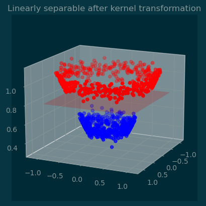

3 Learning Nonlinear Transformation

import sklearn.datasets
import pandas as pd

pl.set_cmap('tab20c')
(x_moon, y_moon) = sklearn.datasets.make_moons(1000, noise=0.1)
pl.scatter(x_moon[:, 0], x_moon[:, 1], c=y_moon, s=1);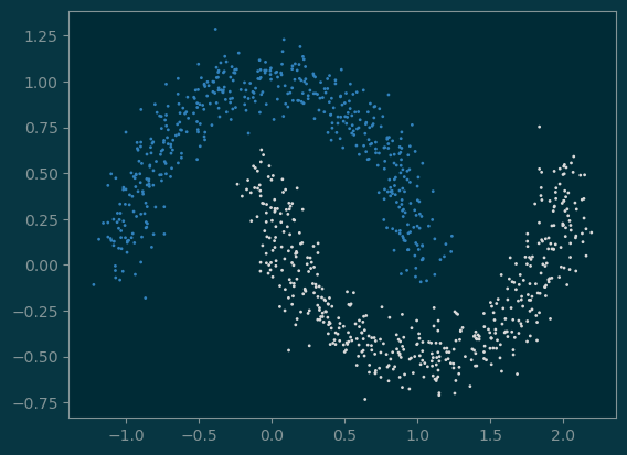

We can incorporate the non-linear kernel transformation as part of the classifier model.

The model now has two layers:

Transform input to a higher dimension:

\[z = \sigma_1(xW_1 + b_1)\] where \(W_1\in\mathbb{R}^{2\times k}\), and \(b_1\in\mathbb{R}^k\) and \(\sigma_1\) can be any non-linear activation function.

Perform classification:

\[ \mathrm{sigmoid}(zW_2 + b_2) \] where \(W_2\in\mathbb{R}^{k}\) and \(b_2\in\mathbb{R}\).

In general, the overall model architecture is given as:

\[ x:\mathrm{Input} \underbrace{\longrightarrow}_\mathrm{hidden} z:k \underbrace{\longrightarrow}_\mathrm{classify} p:c \]

This is known as the multi-linear perceptron (MLP) where

\(k\) is the hidden dimension
\(c\) is the number of classes

4 MLP in PyTorch

import torch
import torch.nn as nn

4.1 The model

class MLPBinaryClassifier(nn.Module):
    def __init__(self, input_dim, hidden_dim):
        super().__init__()
        self.hidden = nn.Linear(input_dim, hidden_dim)
        self.output = nn.Linear(hidden_dim, 1)
        
    def forward(self, x):
        x = self.hidden(x)
        x = nn.functional.softmax(x, dim=1)
        x = self.output(x)
        x = torch.sigmoid(x)
        return x

4.2 Training

x_input = torch.tensor(x_moon, dtype=torch.float32)
y_true = torch.tensor(y_moon, dtype=torch.float32).reshape(-1, 1)

model = MLPBinaryClassifier(2, 10)
optimizer = torch.optim.Adam(model.parameters(), lr=0.1)
loss = nn.functional.binary_cross_entropy

epochs = 10000
for epoch in range(epochs):
    optimizer.zero_grad()
    l = loss(model(x_input), y_true)
    l.backward()
    optimizer.step()
    if epoch % (epochs//10) == 0:
        with torch.no_grad():
            print(epoch, l.numpy())
print(epoch, l.detach().numpy())

0 0.7036692
1000 0.00027156077
2000 7.829278e-05
3000 3.3903292e-05
4000 1.7046508e-05
5000 9.193841e-06
6000 5.150013e-06
7000 2.9483087e-06
8000 1.706474e-06
9000 9.986555e-07
9999 5.871792e-07

4.3 Visualizing classification boundary

x_lim = np.linspace(-1.5, 2.5, 100)
y_lim = np.linspace(-1, 1.5, 100)
xx, yy = np.meshgrid(x_lim, y_lim)
x_input = np.array([xx.ravel(), yy.ravel()]).T
x_input = torch.tensor(x_input, dtype=torch.float32)
x_input.shape

torch.Size([10000, 2])

model.eval()
z = model(x_input)
z = z.reshape(100, 100).detach().numpy()
z.shape

(100, 100)

pl.set_cmap('tab20c')
pl.scatter(x_moon[:, 0], x_moon[:, 1], c=y_moon, s=1)
pl.contour(xx, yy, z, levels=1);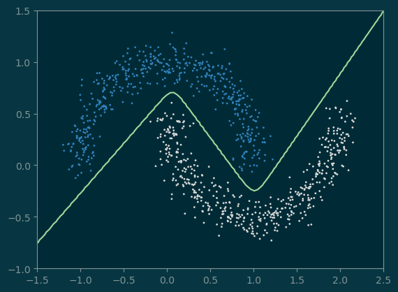

5 PyTorch Sequential Module

class MLP(nn.Module):
    def __init__(self, input_dim, hidden_dim):
        super().__init__()
        self.layers = nn.Sequential(
            nn.Linear(input_dim, hidden_dim),
            nn.Softmax(dim=1),
            nn.Linear(hidden_dim, 1),
            nn.Sigmoid(),
        )
    def forward(self, x):
        return self.layers(x)

#
# train
#

model = MLP(2, 10)
optimizer = torch.optim.Adam(model.parameters(), lr=0.1)
loss = nn.functional.binary_cross_entropy

loss(model(x_input), y_true)

tensor(0.6985, grad_fn=<BinaryCrossEntropyBackward0>)

epochs = 10000
for epoch in range(epochs):
    optimizer.zero_grad()
    l = loss(model(x_input), y_true)
    l.backward()
    optimizer.step()
    if epoch % (epochs//10) == 0:
        with torch.no_grad():
            print(epoch, l.numpy())
print(epoch, l.detach().numpy())

0 0.6985148
1000 0.0004934223
2000 0.00013575741
3000 5.8472422e-05
4000 2.9411138e-05
5000 1.5913067e-05
6000 8.9472505e-06
7000 5.1332345e-06
8000 2.9825378e-06
9000 1.7449648e-06
9999 1.0328644e-06