Optimization Using Gradient ✅

In this section, we will introduce two different topics:

Optimization using gradient based methods.
PyTorch API for managing gradient computation automatically.

import numpy as np
import torch
import matplotlib.pyplot as pl

1 Potential function

A potential function \(f\) is a function mapping from a vector space to a scalar.

\[ f : \mathbb{R}^n \to \mathbb{R} \]

Consider an example of:

\[ f : \mathbb{R}^2 \to \mathbb{R} : (x_1, x_2) \mapsto (x_1^2 + x_2^2) \]

def f(x):
    return x[0] ** 2 + 2 * x[1] ** 2

We can visualize this 2D potential function with a contour plot.

xs = np.linspace(-6, 4, 100)
ys = np.linspace(-6, 4, 100)

xx, yy = np.meshgrid(xs, ys)
coord = np.concatenate([xx[:,:,None], yy[:,:,None]], axis=-1)
coord = coord.reshape(-1, 2).T

z = f(coord)
z = z.reshape(100,100)

pl.set_cmap(pl.get_cmap('jet'))
pl.contourf(xx, yy, z, levels=100)
ax = pl.gca()
ax.set_aspect('equal');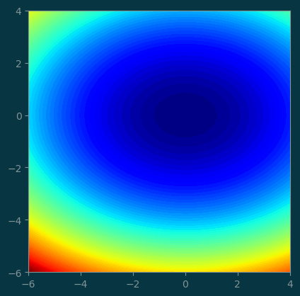

2 Gradient Based Optimization

The gradient of \(f\) is easy to compute by hand:

\[ g= \nabla f(x_1, x_2) = \left[\begin{array}{c} 2x_1 \\ 4x_2 \end{array}\right] \]

def g(x):
    return np.array([2*x[0], 4*x[1]])

Interpretation of gradient

At any particular location \(x_0\in\mathbb{R}^n\), the gradient \((\nabla f)(x_0)\in\mathbb{R}^n\) is a vector.
\((\nabla f)(x_0)\) points to the direction that \(f\) increases at the fastest rate around \(x_0\).
Conversely \(-(\nabla f)(x_0)\) is the direction of the fastest decrease of \(f\) around \(x_0\)
The magnitude of \(|(\nabla f)(x_0)|\) is the rate of change.

3 The Gradient Descent (GD) Minimization Algorithm

The most basic form of the GD algorithm is to following the gradient with small steps.

initialize x to some location
for i in range(num_steps):
    grad = (∇f)(x)
    x = x - step * grad

We need to tune step size.

#
# the GD algorithm that tracks the path
#

def GD(x0, step, num_steps):
    x = np.array(x0)
    history = [[x[0], x[1], f(x)]]
    for i in range(num_steps):
        grad = g(x)
        dx = step * grad
        x = x - dx
        history.append([x[0], x[1], f(x)])
    return np.array(history)

history = GD((-5, -2), step=0.1, num_steps=20)
history.round(1)

array([[-5. , -2. , 33. ],
       [-4. , -1.2, 18.9],
       [-3.2, -0.7, 11.3],
       [-2.6, -0.4,  6.9],
       [-2. , -0.3,  4.3],
       [-1.6, -0.2,  2.7],
       [-1.3, -0.1,  1.7],
       [-1. , -0.1,  1.1],
       [-0.8, -0. ,  0.7],
       [-0.7, -0. ,  0.5],
       [-0.5, -0. ,  0.3],
       [-0.4, -0. ,  0.2],
       [-0.3, -0. ,  0.1],
       [-0.3, -0. ,  0.1],
       [-0.2, -0. ,  0. ],
       [-0.2, -0. ,  0. ],
       [-0.1, -0. ,  0. ],
       [-0.1, -0. ,  0. ],
       [-0.1, -0. ,  0. ],
       [-0.1, -0. ,  0. ],
       [-0.1, -0. ,  0. ]])

pl.contourf(xx, yy, z, levels=100)
pl.plot(history[:, 0], history[:, 1], '-o', color='red')
pl.text(history[-1, 0], history[-1, 1], '%.2f' % history[-1, 2], color='red')
pl.gca().set_aspect('equal');

3.1 Learning rate too small

Selecting the step size is a crucial part of the optimization solution.

Let’s see what happens when the step is too small.

history = GD((-5, -2), step=0.02, num_steps=20)

pl.contourf(xx, yy, z, levels=100)
pl.plot(history[:, 0], history[:, 1], '-o', color='red', markersize=1)
pl.text(history[-1, 0], history[-1, 1], '%.2f' % history[-1, 2], color='red')
pl.gca().set_aspect('equal');

Step size being too small slows the optimization down so much that we didn’t make it to the minimum after 20 steps.

3.2 Step size too large

What happens if we make the step size too large?

history = GD((-5, -2), step=0.48, num_steps=20)

pl.contourf(xx, yy, z, levels=100)
pl.plot(history[:, 0], history[:, 1], '-o', color='red', markersize=5)
pl.text(history[-1, 0], history[-1, 1], '%.2f' % history[-1, 2], color='red')
pl.gca().set_aspect('equal');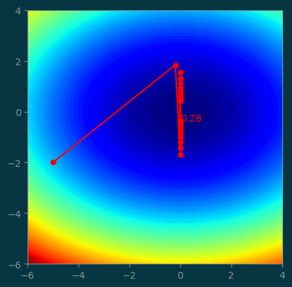

A large step size makes the optimization skip over the minimum, so it keeps isolating around the minimum and never converged.

4 Momentum Based Gradient Optimization

Previously, we have the following:

\[ dx = \mathrm{step}\cdot \nabla(f)(x) \]

In the momentum based GD scheme, we remember the previous \(dx\), and try to keep its direction in the new \(dx\).

\[ dx = \mathrm{step}\cdot \nabla(f)(x) + \mathrm{beta}\cdot dx \]

In the momentum based gradient descent scheme, we maintain a stateful vector called velocity \(\mathbf{v}\in\mathbb{R}^n\).

There are two hyper-parameters: step and beta.

def GD_momentum(x0, step, beta, num_steps):
    x = x0
    dx = [0, 0, ... 0]
    for i in range(num_steps):
        grad = (∇f)(x)
        dx = step * grad + beta * dx
        x = x - dx
    return x

def GD_momentum(x0, step, beta, num_steps):
    x = np.array(x0)
    dx = np.zeros_like(x)
    history = [[x[0], x[1], f(x)]]
    for i in range(num_steps):
        grad = g(x)
        dx = step * grad + beta * dx
        x = x - dx
        history.append([x[0], x[1], f(x)])
    return np.array(history)

4.1 Compare with GD with small steps

history_m = GD_momentum((-5, -2), step=0.02, beta=0.7, num_steps=20)
history = GD((-5, -2), step=0.02, num_steps=20)

pl.contourf(xx, yy, z, levels=100)
pl.plot(history_m[:, 0], history_m[:, 1], '-o', color='yellow', markersize=5)
pl.text(history_m[-1, 0], history_m[-1, 1], '%.2f' % history_m[-1, 2], color='yellow')

pl.plot(history[:, 0], history[:, 1], '-o', color='red', markersize=5)
pl.text(history[-1, 0], history[-1, 1], '%.2f' % history[-1, 2], color='red')

pl.gca().set_aspect('equal');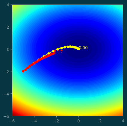

4.2 Comparing with GD with large steps

history_m = GD_momentum((-5, -2), step=0.48, beta=0.7, num_steps=20)
history = GD((-5, -2), step=0.48, num_steps=20)

pl.contourf(xx, yy, z, levels=100)
pl.plot(history_m[:, 0], history_m[:, 1], '-o', color='yellow', markersize=5)
pl.text(history_m[-1, 0], history_m[-1, 1], '%.2f' % history_m[-1, 2], color='yellow')

pl.plot(history[:, 0], history[:, 1], '-o', color='red', markersize=5)
pl.text(history[-1, 0], history[-1, 1], '%.2f' % history[-1, 2], color='red')

pl.gca().set_aspect('equal');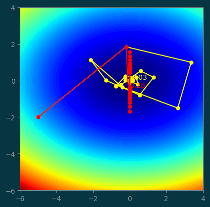

	original	with momentum
0	33.0	33.0
1	6.8	6.8
2	5.7	13.2
3	4.9	11.4
4	4.1	0.4
5	3.5	7.1
6	2.9	1.7
7	2.5	1.6
8	2.1	1.8
9	1.8	0.9
10	1.5	0.3
11	1.3	0.8
12	1.1	0.2
13	0.9	0.2
14	0.8	0.3
15	0.7	0.0
16	0.6	0.1
17	0.5	0.1
18	0.4	0.0
19	0.3	0.0
20	0.3	0.0