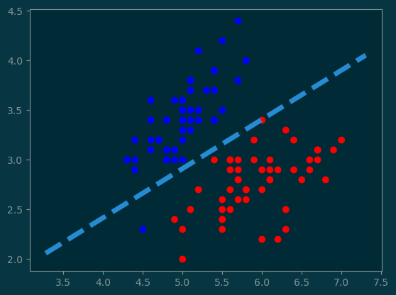
Let’s go through the linear algebra that computes the classification boundary. Since the classification boundary is in \(\mathbb{R}^2\), the boundary is a line.
Logistic regression models the boundary line by the normal vector \(w\) and offset \(b\), and the line is given by: \[
L = \{x\in\mathbb{R}^2: w^Tx + b = 0\}
\]
The nice thing is that this equation for \(L\) generalizes to higher dimensions.
To plot \(L\), we need to transform it into another form:
\[
L = \{x_0 + vt: t\in\mathbb{R}\}
\] where \(x_0, v\in\mathbb{R}^2\).
So, we need to find:
A point already on \(L\): \(x_0\in\mathbb{R}^2\),
the direction vector of \(L\): \(v\in\mathbb{R}^2\).
7.1 Finding a point on \(L\)
Note
Claim:
\(x_0 = -\frac{w}{\|w\|}b\) is on \(L\)
Proof:
Just check:
\[
\begin{eqnarray}
w^T x_0 + b &=& -w^T(\frac{w}{\|w\|^2}b + b \\
&=& -\frac{w^T w}{\|w\|^2}b + b \\
&=& -b + b \\
&=& 0
\end{eqnarray}
\]
7.2 Finding the direction vector of \(L\)
Note
Claim: \[
\left[\begin{array}{c}
u \\
v
\end{array}
\right]^T
\left[\begin{array}{c}
-v \\
u
\end{array}
\right]
= 0
\]
Therefore, given \(w = [w_0, w_1]\), the direction vector is simply \(v = [-w_1, w_0]\).
7.3 Plotting \(L\)
Now that we have: \(L = \{x_0 + vt\}\),
We just need to points:
\(p_1 = x_0 + vt_1\)
\(p_2 = x_0 + vt_2\)
We pick \(t_1\) and \(t_2\) to be two arbitrary values.
plot(
    [p1[0], p2[0]],
    [p1[1], p2[1]], ...)
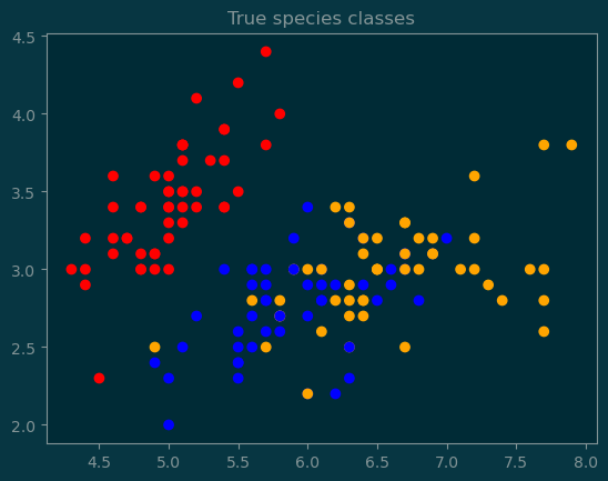
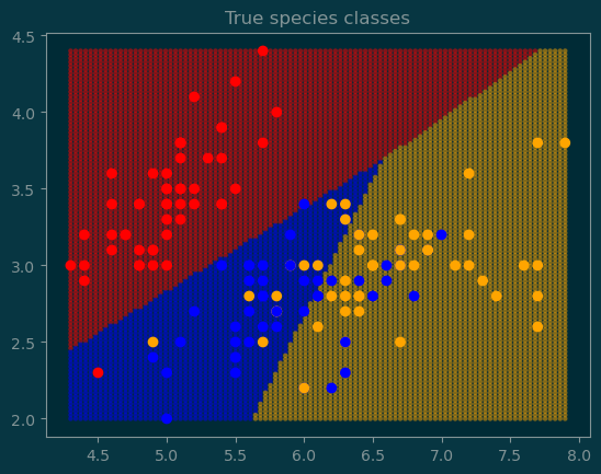
8 Generalizing to multiple classes
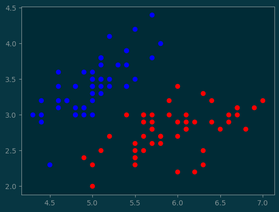
We will now perform classification on all three species based on the sepal length and sepal width.
With multiple classes, the model needs to compute multiple probabilities.
where each \(p_k\) represents the likelihood that \(x\) is the sepal dimensions of species \(k\).
Thus: \(p_1+p_2+p_3 = 1\).
8.1 Logits of classification
The model consists of the model parameters \((W, b)\) where - \(W\in\mathbb{R}^{2\times 3}\) - \(b\in\mathbb{R}^3\).
Given an input \(x\in\mathbb{R}^2\), we have define
\[ v = xW + b \]
From the dimensions, we can tell that \(v\in\mathbb{R}^3\). Here \(v\) is the vector of logits. In order to convert the logits into probabilities, we use the softmax function.
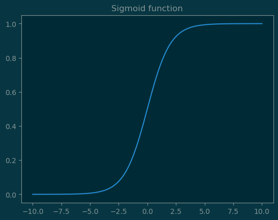
8.2 Softmax function
\[
\mathrm{softmax}:\mathbb{R}^n\to[0,1]^n
\]
For \(p = \mathrm{softmax}(v)\), we have:
\[p_i = \frac{e^{v_i}}{\sum_k e^{v_k}}\]
8.3 A general model
\[
f(x|W,b) = \mathrm{softmax}(xW + b)
\]
Note, \(W\) and \(b\) can be designed to accommodate any input dimension and number of classes.
9 Linear Layer With Activation Function
The model:
\[f(x|W, b) = \mathrm{softmax}(xW + b)\]
is called the linear layer.
The function softmax is called the activation function.
Both are supported by PyTorch.
class Classifier(nn.Module):def__init__(self):super().__init__()self.linear = nn.Linear(2, 3)def forward(self, x):return nn.functional.softmax(self.linear(x), axis=-1)
colormap = {0: 'red',1: 'blue',2: 'orange',}c = [colormap[y] for y in y_true.numpy()]pl.scatter(x_input[:,0], x_input[:, 1], c=c)pl.title('True species classes');
coordinates = X.reshape(-1, 2)for c in [0, 1, 2]: pl.scatter( coordinates[output==c, 0], coordinates[output==c, 1], c=colormap[c], alpha=0.5, edgecolor='none', s=10, )c = [colormap[y] for y in y_true.numpy()]pl.scatter(x_input[:,0], x_input[:, 1], c=c)pl.title('True species classes');