import torch
import torch.nn as nn
import torch.nn.functional as f
import torchvision
import matplotlib.pyplot as plt
reload(my)
<module 'my' from '/workspace/web/my/__init__.py'>import torch
import torch.nn as nn
import torch.nn.functional as f
import torchvision
import matplotlib.pyplot as plt
reload(my)<module 'my' from '/workspace/web/my/__init__.py'>mnist = my.mnist()
cifar10 = my.cifar10()image_1, label_1 = mnist[0]
image_2, label_2 = cifar10[4]image_1.shape, image_2.shape(torch.Size([1, 28, 28]), torch.Size([3, 32, 32]))plt.subplot(1,2,1)
plt.imshow(image_1[0], cmap='gray')
plt.xticks([]); plt.yticks([]);
plt.subplot(1,2,2)
plt.imshow(image_2.permute((1,2,0)))
plt.xticks([]); plt.yticks([]);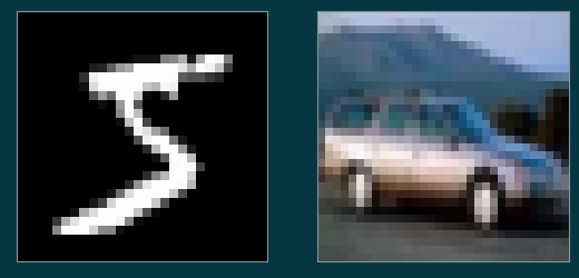
image_2.shapetorch.Size([3, 32, 32])im2 = image_2.permute((1, 2, 0))
plt.figure(figsize=(18, 6))
plt.subplot(1, 4, 1)
plt.imshow(im2)
plt.title('Image 2')
plt.subplot(1, 4, 2)
plt.imshow(im2[:, :, 0], cmap='gray')
plt.title('red')
plt.subplot(1, 4, 3)
plt.imshow(im2[:, :, 1], cmap='gray')
plt.title('green')
plt.subplot(1, 4, 4)
plt.imshow(im2[:, :, 2], cmap='gray')
plt.title('blue');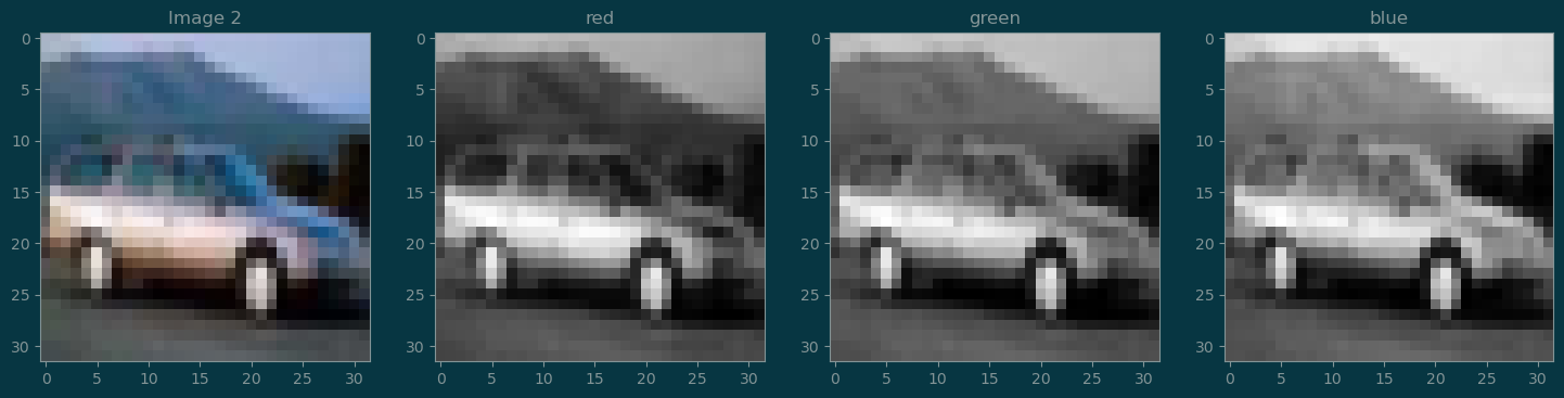
Recall that for vectors, \(x, y\in\mathbb{R}^n\), we can compute their inner product as:
\[ \left<x, y\right> = \sum_{i=1}^n x_i\cdot y_i \]
The two vectors must have the same shape.
This can be generalized to images that have the same shape.
Given two images, \(I_1, I_2\in\mathbb{R}^{c\times h\times w}\), where \(c\) is the channel, and \(w,h\) are the width and height in pixels, their inner product is given as:
\[ \left<I_1, I_2\right> = \sum_{c}\sum_{h}\sum_{w} I_1[k,i,j]\cdot I_2[k,i,j] \]
A patch is a subregion of an image.
image_2.shapetorch.Size([3, 32, 32])(i0, j0) = (20, 16)
s = 10
image = (image_2 * 255).round().type(torch.uint8)
boxes = torch.tensor([(j0,i0,j0+s,i0+s)])
image = torchvision.utils.draw_bounding_boxes(image, boxes, colors='red')
plt.subplot(1, 2, 1)
plt.imshow(image.permute(1, 2, 0))
patch = image_2[:, i0:i0+s, j0:j0+s]
plt.subplot(1, 2, 2)
plt.imshow(patch.permute(1, 2, 0));
Consider an image \(I\) of size \(h\times w\).
Let’s fix the patch size to be \(k\times k\).
Denote the patches by their offsets: \(\mathbf{p}(i,j)\). So, \(\mathbb{p}(i,j)\in\mathbb{R}^{c\times k\times k}\).
The valid range for \(i\) is range(0, h-k+1).
The valide range for \(j\) is range(0, w-k+1).
def overlapping_patches(image, k):
(nchannels, nrows, ncols) = image.shape
patches = torch.zeros((nrows-k+1, ncols-k+1, nchannels, k, k))
for i in range(0, nrows-k+1):
for j in range(0, ncols-k+1):
patches[i,j,:,:,:] = image[:, i:i+k, j:j+k]
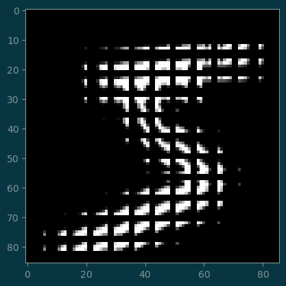
return patchespatches = overlapping_patches(image_1, 5)
patches.shapetorch.Size([24, 24, 1, 5, 5])nrow, _, nchan, h, w = patches.shape
plt.imshow(torchvision.utils.make_grid(patches.reshape((-1, nchan, h, w)), nrow=nrow).permute((1, 2, 0)))
plt.xticks([]); plt.yticks([]);
If we do not allow overlapping, then we need to restrict \((i,j)\) in the patches \(\mathbf{p}(i,j)\) to be:
i in range(0, h-k+1, k)j in range(0, w-k+1, k)This produces \(\mathrm{floor}(h/k) \times \mathrm{floor}(w/k)\) patches.
def nonoverlapping_patches(image, k):
    (nchannels, nrows, ncols) = image.shape
    patches = torch.zeros((nrows // k, ncols // k, nchannels, k, k))
    for i in range(0, nrows-k+1, k):
        for j in range(0, ncols-k+1, k):
            patches[i//k,j//k,:,:,:] = image[:, i:i+k, j:j+k]
    return patches
patches = nonoverlapping_patches(image_1, 5)
patches.shapetorch.Size([5, 5, 1, 5, 5])plt.imshow(
torchvision.utils.make_grid(
patches.reshape(-1, 1, 5, 5),
nrow=5,
).permute(1, 2, 0),
cmap='gray',
)<matplotlib.image.AxesImage at 0x7fde991c9d80>
def strided_patches(image, k, stride):
    (nchannels, h_in, w_in) = image.shape
    h_out = (h_in - k) // stride + 1
    w_out = (w_in - k) // stride + 1
    patches = torch.zeros(h_out, w_out, nchannels, k, k)
    for (i_out, i) in enumerate(range(0, h_in-k+1, stride)):
        for (j_out, j) in enumerate(range(0, w_in-k+1, stride)):
            patches[i_out, j_out,:,:,:] = image[:, i:i+k, j:j+k]
    return patches
patches = strided_patches(image_1, 5, 2)
patches.shapetorch.Size([12, 12, 1, 5, 5])plt.imshow(
torchvision.utils.make_grid(
patches.reshape(-1, 1, 5, 5),
nrow=12,
).permute(1, 2, 0),
cmap='gray',
);
A kernel is a pattern we want to search in the patches of an image.
Convolution involves:
\[ \mathrm{conv}(I, K)[i,j] = \left<\mathbf{p}(i,j), K\right> \]
#
# kernel size = 8
#
kernel_size = 8
kernel = image_1[:, 10:10+kernel_size, 10:10+kernel_size]

plt.subplot(1, 2, 1)
plt.imshow(image_1[0], cmap='gray')

plt.subplot(1, 2, 2)
plt.imshow(kernel[0], cmap='gray')
plt.xticks([]); plt.yticks([]);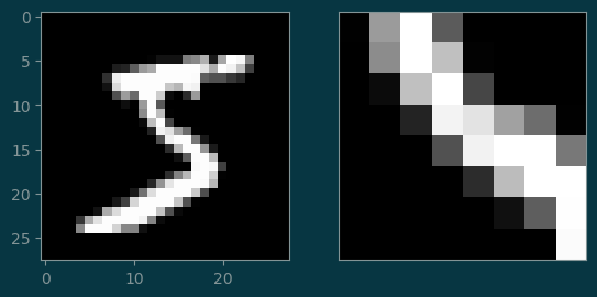
conv2d = torch.nn.functional.conv2dresult = conv2d(
image_1.reshape((1, 1, 28, 28)),
kernel.reshape(1, 1, kernel_size, kernel_size),
)
result.shapetorch.Size([1, 1, 21, 21])plt.imshow(result[0,0], cmap='jet')
plt.xticks([]); plt.yticks([]);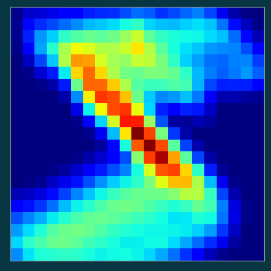
kernel_size = 8
kernel_1 = image_1[:, 10:10+kernel_size, 10:10+kernel_size]
kernel_2 = image_1[:, 20:20+kernel_size, 5:5+kernel_size]
plt.subplot(1, 3, 1)
plt.imshow(image_1[0], cmap='gray')
plt.subplot(1, 3, 2)
plt.imshow(kernel_1[0], cmap='gray')
plt.xticks([]); plt.yticks([]);
plt.subplot(1, 3, 3)
plt.imshow(kernel_2[0], cmap='gray')
plt.xticks([]); plt.yticks([]);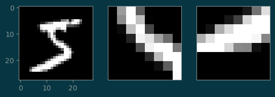
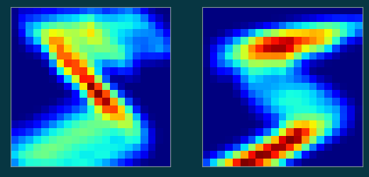
result = conv2d(
image_1.reshape(1, 1, 28, 28),
torch.stack([kernel_1, kernel_2]),
)
result.shapetorch.Size([1, 2, 21, 21])plt.subplot(1, 2, 1)
plt.imshow(result[0,0], cmap='jet')
plt.xticks([]); plt.yticks([]);
plt.subplot(1, 2, 2)
plt.imshow(result[0,1], cmap='jet')
plt.xticks([]); plt.yticks([]);