import torch
import matplotlib.pyplot as pl
import numpy as npRegression ✅
1 The data
x = torch.linspace(0, 1, 10)
y_true = 3 * x + torch.sin(6 * x) + 1
pl.plot(x, y_true, '--o');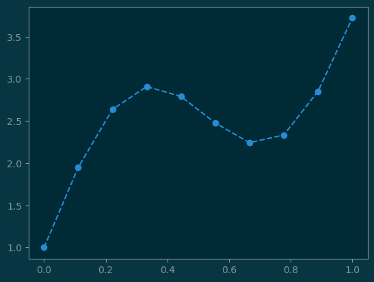
2 A model
We start with a model that relates \(y\) with the input \(x\).
\[ y = f(x | W) \]
where \(W\) is one or more tunable parameters. In the case of linear regression, we have \(W=[a, b]\) such that
\[ f(x|W) = ax + b \]
Given some weights \(W = (a, b)\), we can assess how well the model fits the true values of \(y\) by computing the error:
\[ \mathrm{err} = \frac{\sum_{i}|y_i - f(x_i|W)|^2}{n} \]
Basically, we have:
\[ \mathrm{err} : W \mapsto \mathbb{R} \]
The error function can help us to improve the model by computing the gradient with respect to \(W\).
\[ W' = W - \epsilon\cdot \nabla\mathrm{err} \]
Theorem
For sufficiently small \(\epsilon\), we are guaranteed to have \(\mathrm{err}(W') < \mathrm{err}(W)\)
3 PyTorch Model
W = torch.tensor([0., 0.], requires_grad=True)y_pred = W[0]*x + W[1]err = torch.linalg.vector_norm(y_pred - y_true) / x.shape[0]
errtensor(0.8162, grad_fn=<DivBackward0>)err.backward()grad = W.grad
gradtensor([-0.1710, -0.3053])3.1 Update the weights with a step
Let’s update the weights with a small step size:
\[ W_{n+1} = W_{n} - \epsilon\cdot \nabla\mathrm{err} \]
epsilon = 0.01
with torch.no_grad():
W.sub_(epsilon * grad)
Wtensor([0.0017, 0.0031], requires_grad=True)Q: Why do we need with torch.no_grad()?
A: By default, any computation that involves \(W\) will trigger a gradient propagation. But \(W \to W-\epsilon\cdot\nabla\mathrm{err}\) is not part of model computation, but rather the optimization computation. So, we have to disable the gradient tracking.
#
# Previous error is 0.8162
#
y_pred = W[0]*x + W[1]
err = torch.linalg.vector_norm(y_pred - y_true) / x.shape[0]
errtensor(0.8150, grad_fn=<DivBackward0>)3.2 One more gradient update
W.grad.zero_()

err.backward()
grad = W.grad

with torch.no_grad():
    W.sub_(epsilon * grad)

W
tensor([0.0034, 0.0061], requires_grad=True)Q: Why do we need W.grad.zero_()?
A: The exact action of err.backward() is to accumulate the gradient to the existing W.grad. So, by default, it will retain the gradient value from the previous update. Since we only care about the gradient from the current error, we need to clear W.grad before err.backward().
#
# Previous error is 0.8150
#

y_pred = W[0]*x + W[1]
err = torch.linalg.vector_norm(y_pred - y_true) / x.shape[0]
err
tensor(0.8138, grad_fn=<DivBackward0>)4 A training loop
def init(W):
    with torch.no_grad():
        W.zero_()
def err(W):
y = W[0] * x + W[1]
return torch.linalg.norm(y - y_true) / x.shape[0]def update_step():
W.grad.zero_()
e = err(W)
e.backward()
with torch.no_grad():
W.sub_(epsilon * W.grad)
return e.detach().item()def report(i):
with torch.no_grad():
e = err(W)
print("[{}] a={:.2f} b={:.2f}, err={:.2f}".format(i, W[0], W[1], e))N = 2000
e = np.zeros(N)
init(W)
for i in range(N):
e[i] = update_step()
if i % (N//10) == 0:
report(i)
report(N)[0] a=0.00 b=0.00, err=0.81
[200] a=0.34 b=0.61, err=0.57
[400] a=0.67 b=1.19, err=0.35
[600] a=0.96 b=1.66, err=0.20
[800] a=1.12 b=1.87, err=0.16
[1000] a=1.17 b=1.90, err=0.16
[1200] a=1.21 b=1.90, err=0.15
[1400] a=1.23 b=1.88, err=0.15
[1600] a=1.26 b=1.87, err=0.15
[1800] a=1.28 b=1.86, err=0.15
[2000] a=1.30 b=1.85, err=0.155 Fitting the data
(a, b) = W.detach().numpy()

y_pred = a * x + b
Q: Why do we need W.detach()?
A: This is another way to avoid triggering gradient computation on W. Basically W.detach() takes a snapshot of W by making a copy of it. The copy will not participate in the gradient computation.
pl.subplot(2,1,1)
pl.plot(x, y_true, '--')
pl.plot(x, y_pred, '-');

pl.subplot(2,1,2)
pl.plot(e);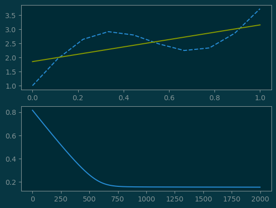
6 PyTorch API
class LineFitting(torch.nn.Module):
    def __init__(self):
        super().__init__()
        W = torch.tensor([0, 0], dtype=torch.float32)
        self.W = torch.nn.Parameter(W)
        self.length = x
    def forward(self, x):
        return self.W[0] * x + self.W[1]
#
# The model can be used as a function to evaluate the forward computation
#
line = LineFitting()
line(x)tensor([0., 0., 0., 0., 0., 0., 0., 0., 0., 0.], grad_fn=<AddBackward0>)def train(x, y_true, model, LossFn, OptimizerFn, lr, epochs):
loss = LossFn()
optimizer = OptimizerFn(model.parameters(), lr=lr)
for epoch in range(epochs):
optimizer.zero_grad()
y = model(x)
loss(y, y_true).backward()
optimizer.step()
if epoch % (epochs//10) == 0:
with torch.no_grad():
l = loss(y, y_true).numpy()
W = next(model.parameters()).numpy()
print(l, W)train(x, y_true, line, torch.nn.MSELoss, torch.optim.SGD, 0.1, 10)6.661948 [0.27913672 0.49835616]
3.8140697 [0.48879483 0.8691274 ]
2.2304645 [0.6466221 1.1447786]
1.3497871 [0.76577795 1.3495169 ]
0.8599378 [0.85607487 1.5013919 ]
0.58739096 [0.9248301 1.6138622]
0.4356683 [0.97749996 1.6969628 ]
0.35112858 [1.0181533 1.7581764]
0.30394772 [1.0498246 1.803082 ]
0.27754354 [1.0747765 1.8358393]def plot(x, y_true, model):
with torch.no_grad():
y = model(x)
pl.plot(x, y_true, '--o')
pl.plot(x, y, '-');plot(x, y_true, line)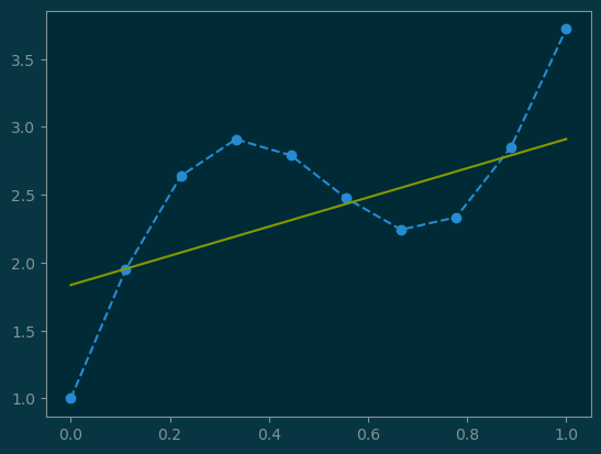
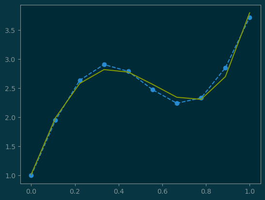
7 Fitting using power series
Let’s consider the following model:
\[ y_i = \sum_{k=0}^n w_k\cdot x_i^k \]
class PolyFit(torch.nn.Module):
    def __init__(self, degree):
        super().__init__()
        self.degree = degree
        self.W = torch.nn.Parameter(torch.zeros(degree))

    def forward(self, x):
        y = torch.zeros_like(x)
        for i in range(self.degree):
            y += self.W[i] * (x ** i)
        return y
poly = PolyFit(5)train(x, y_true, poly, torch.nn.MSELoss, torch.optim.SGD, 0.05, 100_000)6.661948 [0.24917808 0.13956836 0.10177316 0.08296516 0.07186685]
0.096582726 [ 1.5249301 4.626327 -5.4320383 -1.7490873 4.497506 ]
0.0407205 [ 1.3294919 6.8686876 -9.060711 -2.8561032 7.314907 ]
0.019431062 [ 1.2087605 8.256573 -11.31992 -3.5080438 9.038196 ]
0.011308028 [ 1.1341342 9.117172 -12.734032 -3.8792846 10.086427 ]
0.008199797 [ 1.087948 9.652406 -13.626566 -4.0774508 10.718156 ]
0.007001873 [ 1.0593315 9.986803 -14.197132 -4.1690907 11.093055 ]
0.006531924 [ 1.0415397 10.197327 -14.569023 -4.194967 11.309404 ]
0.0063396967 [ 1.0304453 10.331186 -14.817809 -4.180671 11.428036 ]
0.0062534497 [ 1.0234796 10.417755 -14.990616 -4.1417074 11.486474 ]plot(x, y_true, poly);