Linear Algebra ✅

import numpy as np
import matplotlib.pyplot as pl
from mpl_toolkits.mplot3d import Axes3D

1 Vectors

1.1 A single vector

#
# A 2D vector
#

v = np.array([1, 2])
v

array([1, 2])

#
# We can plot it in an 2D plot as a point
#

pl.scatter([v[0]], [v[1]], s=100)
pl.grid(True)
pl.xlim((-5, 5))
pl.ylim((-5, 5));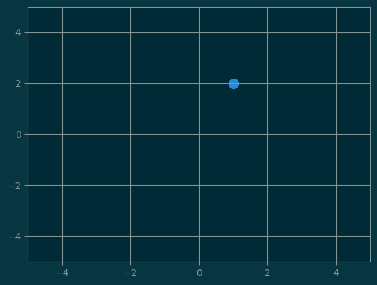

1.2 Higher dimensional vector

v = np.array([1, 2, 3])
v

array([1, 2, 3])

#
# We can plot it in a 3D grid
#
fig = pl.figure()
ax = fig.add_subplot(projection='3d')
ax.set_xlim(-5, 5)
ax.set_ylim(-5, 5)
ax.set_zlim(-5, 5)
ax.scatter([v[0]], [v[1]], [v[2]], s=100);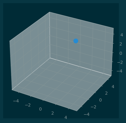

1.3 A collection of vectors

x_list = np.random.normal(0, 1, size=(1000,))
y_list = np.random.normal(0, 2, size=(1000,))
v_list = np.vstack([x_list, y_list])

pl.figure(figsize=(6,6))
pl.xlim((-10, 10))
pl.ylim((-10, 10))

pl.scatter(v_list[0, :], v_list[1, :], s=1);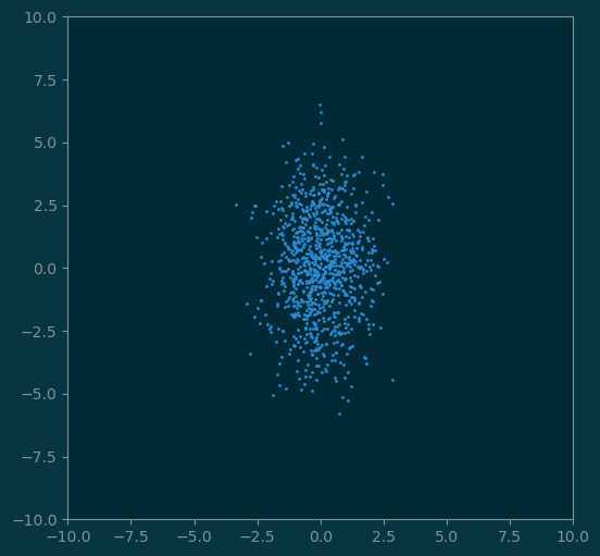

2 Matrices

Matrix construction
Transpose
Multiplication
Rotational matrices

2.1 Constructing matrices

#
# We construct matrices using nested Python arrays
#

M = np.array([
    [1, 2, 3],
    [4, 5, 6]
])

M

array([[1, 2, 3],
       [4, 5, 6]])

2.2 Transpose and multiplication

#
# We can apply matrix transformations.
#

np.transpose(M)

array([[1, 4],
       [2, 5],
       [3, 6]])

#
# We can apply matrix transformations.
#

M.T

array([[1, 4],
       [2, 5],
       [3, 6]])

#
# Matrix multiplication is done by `@` operator
#

X = np.ones((4, 2))

X @ M

array([[5., 7., 9.],
       [5., 7., 9.],
       [5., 7., 9.],
       [5., 7., 9.]])

2.3 Scaling Matrices

t = np.linspace(0, 2 * np.pi, 20)
xs = 2*np.cos(t)
ys = np.sin(t)

points = np.vstack([xs, ys])

def show(*args):
    pl.figure(figsize=(6,6))
    pl.grid(True)
    pl.xlim(-5, 5)
    pl.ylim(-5, 5);
    for i in range(0, len(args), 2):
        points = args[i]
        color = args[i+1]
        xs = points[0]
        ys = points[1]
        pl.scatter(xs, ys, s=100, color=color)

show(points, 'gray')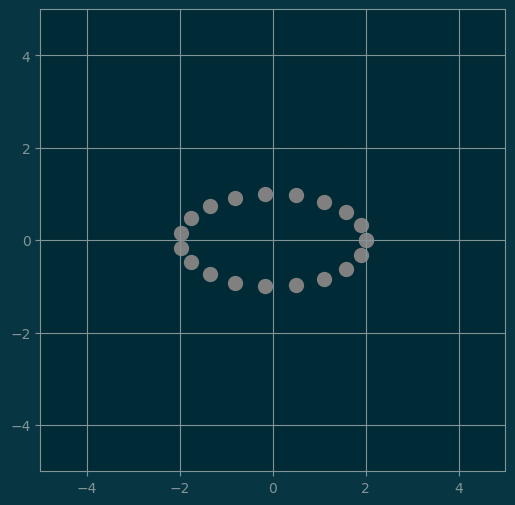

M1 = np.array([
    [2, 0],
    [0, 2]
])

new_points = M1 @ points

show(points, 'gray', new_points, 'blue')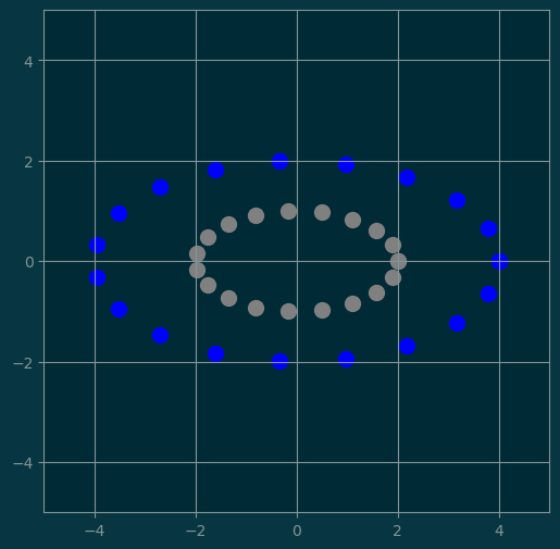

M2 = np.array([
    [0.5, 0],
    [0, 1.5]
])

show(points, 'gray', M2 @ points, 'blue')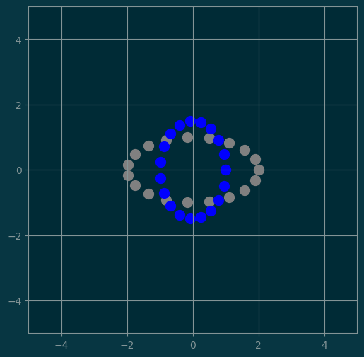

3 Rotational matrix

def rotation_M(theta):
    return np.array([
        [np.cos(theta), np.sin(theta)],
        [-np.sin(theta), np.cos(theta)]
    ])

M3 = rotation_M(np.pi/4)
show(points, 'gray', M3 @ points, 'blue')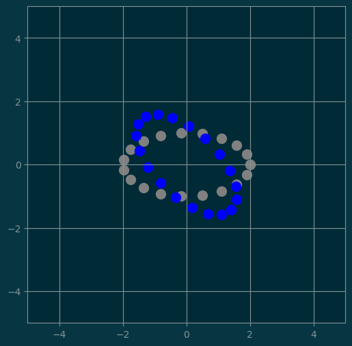

3.1 Composition of transformations

#
# We can compose the matrices together
#

M4 = M3 @ M2 @ M1

show(points, 'gray', M4 @ points, 'blue')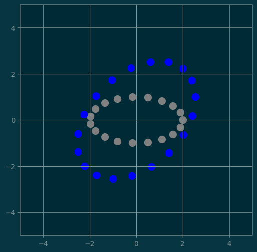

#
# We can compose the matrices together
#

show(points, 'gray', M1 @ M2 @ M3 @ points, 'blue')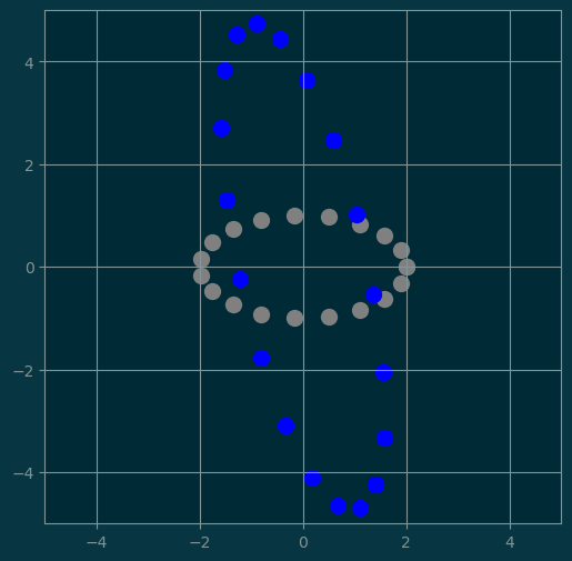

4 Distances

Inner product (or dot product)
Vector norms
Distance as a norm
Cosine similarity

4.1 Inner product

x = np.array([1, 2])
y = np.array([3, 4.5])
z = np.array([0, 2])

pl.figure(figsize=(6,6))
pl.xlim(-6, 6)
pl.ylim(-6, 6)
pl.grid(True)
pl.text(x[0], x[1], 'x', fontsize=24)
pl.text(y[0], y[1], 'y', fontsize=24)
pl.text(z[0], z[1], 'z', fontsize=24)
pl.scatter([0], [0], s=200);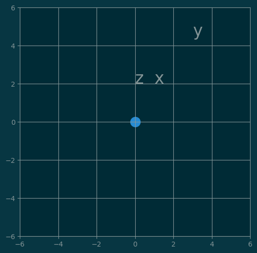

#
# Inner product
#

a = np.dot(x, y)
a

12.0

x @ y

12.0

4.2 Norm of a vector

The norm of a vector \(x\) is its length, denoted by \(\|x\|\).

It can be computed as:

\[\left<x, x\right> = \|x\|^2 \]

Thus,

\[ \|x\| = \sqrt{\left<x, x\right>} \]

np.sqrt(x @ x)

2.23606797749979

np.sqrt(y @ y)

5.408326913195984

np.sqrt(z @ z)

2.0

4.3 Distance

\[ d(x, y) = \|x - y\| \]

def d(x, y):
    v = x - y
    return np.sqrt(v @ v)

#
# Distance is the norm of the difference vector
#

d(x, y)

3.2015621187164243

# Distance is symmetric

d(y, x)

3.2015621187164243

d(x, z)

1.0

d(y, z)

3.905124837953327

points = np.array([x, y, z])
points

array([[1. , 2. ],
       [3. , 4.5],
       [0. , 2. ]])

import scipy.spatial
scipy.spatial.distance_matrix(points, points)

array([[0.        , 3.20156212, 1.        ],
       [3.20156212, 0.        , 3.90512484],
       [1.        , 3.90512484, 0.        ]])

4.4 Cosine similarity

\[ \cos(\theta) = \frac{\left<x, y\right>}{ \|x\| \|y\|} \]

def sim(x, y):
    return (x @ y) / np.sqrt(x @ x) / np.sqrt(y @ y)

sim(x, x)

1.0

sim(x, y)

0.9922778767136676

sim(x, z)

0.8944271909999159

np.arccos(sim(x, x))

0.0

np.arccos(sim(x, y)) * 180 / np.pi

7.1250163489018075

np.arccos(sim(x, z)) * 180 / np.pi

26.56505117707799

4.5 Projection

Did you know that the projection of some vector \(u\) onto another vector \(v\) is given by:

Make \(v\) into a unit vector:

\[ v \mapsto \frac{v}{\|v\|} \]
Compute the length of projection:

\[\begin{eqnarray*} \mathbf{proj}(u, v) &=& \cos(\theta)\|u\| v \\ &=& \frac{\left<u, v\right>} {\|u\|\|v\|} \|u\|v \\ &=& \left<u, v\right> v \end{eqnarray*}\]

def proj(u, v):
    v = v / np.sqrt(v @ v)
    return u @ v * v

u = np.array([1, 1])
v = np.array([1, 2])
w = proj(u, v)

w

array([0.6, 1.2])

pl.figure(figsize=(6,6))
pl.xlim(0, 2.5)
pl.ylim(0, 2.5)
pl.arrow(0, 0, u[0], u[1], head_width=0.04, width=0.01, color='gray');
pl.arrow(0, 0, v[0], v[1], head_width=0.04, width=0.02, color='green');
pl.arrow(0, 0, w[0], w[1], head_width=0.04, width=0.01, color='red');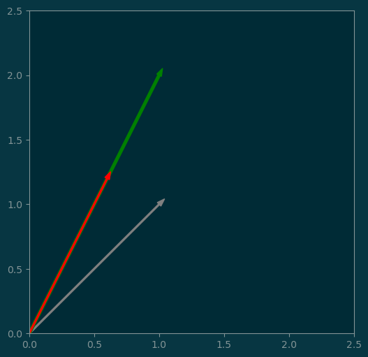

5 Lines and Planes

5.1 Line through the origin

\[L_u = \{ cu : c\in\mathbb{R} \}\]

def line(u):
    c = np.linspace(-10, 10, 20)
    return c[:, np.newaxis] @ u[np.newaxis, :]

u = np.array([1, 1])
points = line(u)
pl.grid(True)
pl.scatter(0, 0, s=200)
pl.scatter(points[:, 0], points[:, 1], s=50);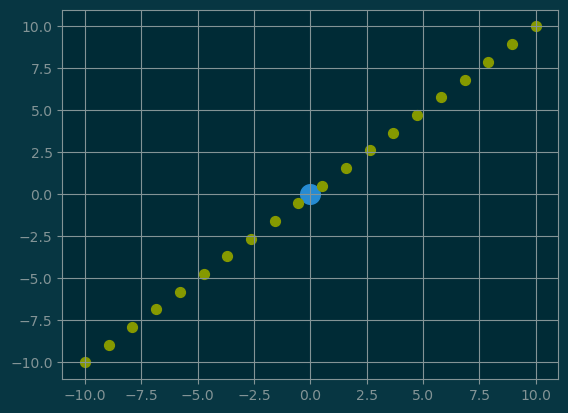

5.2 Line not through the origin

\[ L_{u, b} = \{ cu + b: c\in\mathbb{R} \}\]

def line_offset(u, b):
    return line(u) + b

u = np.array([1, 1])
b = np.array([0, -5])
points = line_offset(u, b)

pl.grid(True)
pl.scatter(0, 0, s=200)
pl.scatter(b[0], b[1], s=100)
pl.scatter(points[:, 0], points[:, 1], s=50);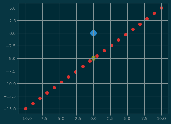

5.3 Plane through the origin

\[P_{u,v} = \{ au + bv: a\in\mathbb{R}, b\in\mathbb{R} \}\]

def plane(u, v):
    a_line = line(u) # (n, 3)
    b_line = line(v) # (n, 3)
    grid = a_line[:, np.newaxis, :] + b_line[np.newaxis, :, :]
    return grid

u = np.array([-0.35606907, -0.45829173,  0.8143608 ])
v = np.array([ 0.73476628, -0.675748  , -0.05901828])
P = plane(u, v)
P.shape

(20, 20, 3)

fig = pl.figure(figsize=(6,6))
ax = fig.add_subplot(projection='3d')
ax.set_xlim(-5, 5)
ax.set_ylim(-5, 5)
ax.set_zlim(-5, 5)
points = P.reshape(-1, 3)
ax.scatter(points[:, 0], points[:, 1], points[:, 2], s=10);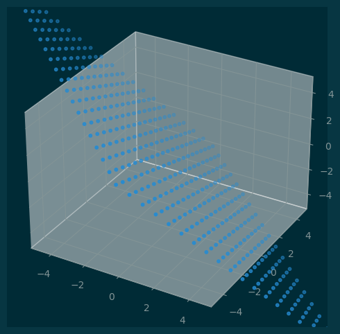

5.4 Plane defined by normal vector

Given a vector \(w\),

\[P_w = \{ x\in\mathbb{R}^k : \left<x, w\right> = 0 \}\]

We can translate the definition of a plane between the normal vector \(w\), and its two spanning vectors \(u, v\).

#
# Given a vector
#

w = np.array([2, 3, 4])
w

array([2, 3, 4])

#
# We can find an orthogonal vector
#

def get_normal_vector(w):
    rand = np.random.random(3)
    rand_proj = proj(rand, w)
    return rand - rand_proj

print("w =", w)
print("normal to w =", get_normal_vector(w))
print("sim(u, w) =", sim(w, get_normal_vector(w)))

w = [2 3 4]
normal to w = [ 0.1282955   0.38550103 -0.35327353]
sim(u, w) = 3.649751635494471e-16

#
# We can find an orthogonal vector from two known vectors: u, w
#

v = np.cross(w, get_normal_vector(w))
print("v =", v)
print("sim(v, w) =", sim(v, w))

v = [ 0.87744265  1.78406671 -1.77677136]
sim(v, w) = 0.0

6 Projection and Separation

Projection on to a line
Projection on to a plane
Separation by a plane

6.1 Projection onto a line

Let \(L_u\) be a line through the origin, defined by a direction vector \(u\).

Let \(v\) be any vector. We can compute the projection of \(v\) on \(L_u\).

\[\mathbf{proj}_L(v) = \mathbf{proj}(v, u)\]

u = np.array([1, 2])
v = np.array([-10, 15])
w = proj(v, u)

points = line(u)
pl.figure(figsize=(6,6))
pl.grid(True)
pl.xlim(-20, 20)
pl.ylim(-20, 20)
pl.scatter(points[:, 0], points[:, 1], s=20);
pl.scatter(v[0], v[1], color='red', s=150);
pl.scatter(w[0], w[1], color='red', s=50);

6.2 Projection on a line revisited

Consider \(L_u\) being a line through the origin, defined by vector \(u\).

Let \(v\) be a vector. The projection of \(v\) onto \(L\) can be computed by a normal vector of \(L\).

Let \(t\) be a vector, normal to \(u\). Namely,

\[ \left<t, u\right> = 0 \]

Then, we have the following relation:

\[ v = \mathbf{proj}(v, t) + \mathbf{proj}(v, u) \]

Therefore, the projection on the line is given by:

\[ \mathbf{proj}(v, L_u) = \mathbf{proj}(v, u) = v - \mathbf{proj}(v, t) \]

u = np.array([1, 2])
t = np.array([-2, 1])

v = np.array([-10, 15])
w = v - proj(v, t)

points = line(u)
pl.figure(figsize=(6,6))
pl.grid(True)
pl.xlim(-20, 20)
pl.ylim(-20, 20)
pl.scatter(points[:, 0], points[:, 1], s=20);
pl.scatter(v[0], v[1], color='red', s=150);
pl.scatter(w[0], w[1], color='red', s=50);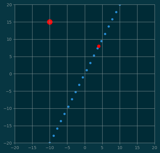

6.3 Projection on to a plane

Consider a plan \(P_t\) through the origin, defined by its normal vector \(t\).

Let \(v\) be a vector. The projection of \(v\) onto \(P_u\) is given by:

\[ \mathbf{proj}(v, P) = v - \mathbf{proj}(v, t) \]

#
# The plane
#
t = np.array([1, 1, 1])
a = get_normal_vector(t)
a = a / np.sqrt(a @ a)
b = np.cross(t, a)
b = b / np.sqrt(b @ b)
points = plane(a, b).reshape(-1, 3)

#
# The point
#
v = np.array([5, 0, 2])

#
# The projection of v onto the plane
#
w = v - proj(v, t)

print("w is normal to t: ", sim(w, t))

fig = pl.figure(figsize=(6,6))
ax = fig.add_subplot(projection='3d')
ax.set_xlim(-5, 5)
ax.set_ylim(-5, 5)
ax.set_zlim(-5, 5)
ax.scatter(points[:, 0], points[:, 1], points[:, 2], s=10);
ax.scatter(v[0], v[1], v[2], s=100, color='red');
ax.scatter(w[0], w[1], w[2], s=30, color='red');

w is normal to t:  -2.881631309228584e-16

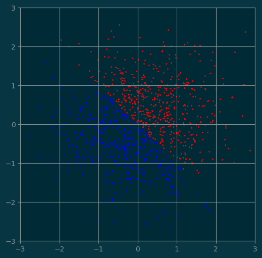
6.4 Planar separation

Let \(P_t\) be a plane through the origin, defined by its normal vector \(t\).

The plane divides the whole space into two partitions.

Above the plane: \[ \{x\in\mathbb{R}^n: \left<x, t\right> > 0\} \]
Below the plane: \[ \{x\in\mathbb{R}^n: \left<x, t\right> < 0\} \]

X = np.random.randn(1000, 2)

pl.figure(figsize=(6,6))
pl.xlim(-3, 3)
pl.ylim(-3, 3)
pl.grid(True)
pl.scatter(X[:, 0], X[:, 1], s=1);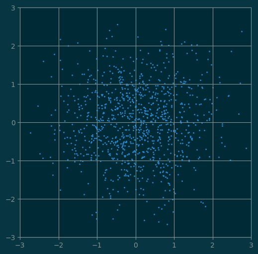

t = np.array([1, 1])

I = X @ t > 0
J = X @ t < 0

pl.figure(figsize=(6,6))
pl.xlim(-3, 3)
pl.ylim(-3, 3)
pl.grid(True)
pl.scatter(X[I, 0], X[I, 1], s=1, color='red')
pl.scatter(X[J, 0], X[J, 1], s=1, color='blue');