import torch
import torchvision
import matplotlib.pyplot as pl
import numpy as npMachine Learning Workflow ✅
1 Dataset
A dataset is a large collection of input-output pairs: \(\{(x_i, y_i): i\in D\}\). Each pair \((x, y)\) is called a sample.
The dataset is to be used for both training and testing of a machine learning system.
For neural network based training, we have to encode everything as tensors. Thus, each sample must be transformed into some tensor of real numbers.
For numerical reasons, we want the rescale the numerical value to values close to \([-1, 1]\).
1.1 PyTorch datasets
PyTorch provides a set of standard datasets for educational and research purposes.
from torchvision import transforms

transform = transforms.Compose([
    transforms.ToTensor(),
])

dataset = torchvision.datasets.mnist.MNIST('/workspace/datasets/', download=True, transform=transform)
1.2 The MNIST dataset
#
# The input data is 28x28 tensor of integers.
#
dataset.data.shape, dataset.data.dtype
(torch.Size([60000, 28, 28]), torch.uint8)#
# The output data is just integers.
#
dataset.targets.shape, dataset.targets.dtype(torch.Size([60000]), torch.int64)Let’s inspect the data as an image.
x, y = dataset[0]
x.shape, type(y)
(torch.Size([1, 28, 28]), int)x.squeeze_()
pl.imshow(x, cmap='gray')
pl.xticks([]); pl.yticks([])
pl.title(f'Label = {y}');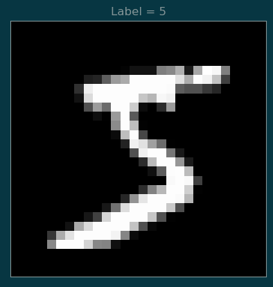
fig = pl.figure(figsize=(6,4))

for i in range(12):
    x, y = dataset[i]
    ax = fig.add_subplot(3,4,i+1)
    ax.set_aspect('equal')
    ax.set_xticks([])
    ax.set_yticks([])
    ax.imshow(x.squeeze(), cmap='gray')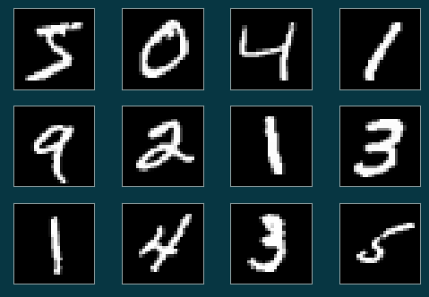
2 Data loader
Data loader is a stage of the machine learning pipeline that feeds data into the neural networks.
Shuffle dataset samples into pseudo random positions to avoid bad gradient estimation.
Split dataset samples into small batches during stochastic gradient descent training.
PyTorch provides a helper class to perform data loading.
dataloader = torch.utils.data.DataLoader(dataset, batch_size=36, shuffle=True)for (xs, ys) in dataloader:
break
xs.shape, ys.shape(torch.Size([36, 1, 28, 28]), torch.Size([36]))im = torchvision.utils.make_grid(xs, nrow=6)
pl.imshow(np.transpose(im, (1,2,0)))
pl.xticks([])
pl.yticks([]);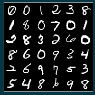
3 Neural Network Model
Now we can build the model and optimizer for training.
3.1 A MLP model
from torch import nnclass MyModel(nn.Module):
def __init__(self):
super().__init__()
self.net = nn.Sequential(
nn.Flatten(),
nn.Linear(28*28, 100),
nn.ReLU(),
nn.Linear(100, 10)
)
def forward(self, x):
return self.net(x)model = MyModel()3.2 The loss function
loss_fn = nn.CrossEntropyLoss()3.3 Optimizer
optimizer = torch.optim.Adam(model.parameters())4 Training
def train(model, optimizer, loss_fn, epochs):
    for epoch in range(epochs):
        for (i, (x, y_true)) in enumerate(dataloader):
            optimizer.zero_grad()
            y_out = model(x)
            loss = loss_fn(y_out, y_true)
            loss.backward()
            optimizer.step()
            if i % 100 == 0:
                report(model, dataset, loss_fn)
        report(model, dataset, loss_fn)

def report(model, dataset, loss_fn):
    with torch.no_grad():
        length = len(dataset)
        for x, y_true in torch.utils.data.DataLoader(dataset, batch_size=length):
            y_out = model(x)
            loss = loss_fn(y_out, y_true).item()
            y_pred = y_out.argmax(axis=1)
            success = (y_pred == y_true).sum().item()
            accuracy = success / length
            print(f"Loss = {loss:.2f}, Accuracy = {accuracy:.2f}")
train(model, optimizer, loss_fn, epochs=1)Loss = 2.28, Accuracy = 0.22
Loss = 0.51, Accuracy = 0.86
Loss = 0.38, Accuracy = 0.89
Loss = 0.33, Accuracy = 0.90
Loss = 0.31, Accuracy = 0.91
Loss = 0.29, Accuracy = 0.91
Loss = 0.26, Accuracy = 0.92
Loss = 0.25, Accuracy = 0.93
Loss = 0.25, Accuracy = 0.93
Loss = 0.23, Accuracy = 0.93
Loss = 0.22, Accuracy = 0.93
Loss = 0.20, Accuracy = 0.94
Loss = 0.19, Accuracy = 0.95
Loss = 0.19, Accuracy = 0.94
Loss = 0.18, Accuracy = 0.95
Loss = 0.17, Accuracy = 0.95
Loss = 0.16, Accuracy = 0.95
Loss = 0.16, Accuracy = 0.955 Model Evaluation
test_dataset = torchvision.datasets.MNIST('/workspace/datasets/', train=False, transform=transform)
test_dataloader = torch.utils.data.DataLoader(test_dataset, batch_size=len(test_dataset))model.eval()
report(model, test_dataset, loss_fn)Loss = 0.16, Accuracy = 0.956 Model In Production
for k, v in model.state_dict().items():
    print(k, v.shape)
net.1.weight torch.Size([100, 784])
net.1.bias torch.Size([100])
net.3.weight torch.Size([10, 100])
net.3.bias torch.Size([10])6.1 Saving model to disk
torch.save(model.state_dict(), './model_params.pt')6.2 Loading model from disk
model_state_dict = torch.load('./model_params.pt')

model_in_prod = MyModel()
model_in_prod.load_state_dict(model_state_dict)
<All keys matched successfully>model_in_prodMyModel(
(net): Sequential(
(0): Flatten(start_dim=1, end_dim=-1)
(1): Linear(in_features=784, out_features=100, bias=True)
(2): ReLU()
(3): Linear(in_features=100, out_features=10, bias=True)
)
)report(model_in_prod, test_dataset, loss_fn)Loss = 0.16, Accuracy = 0.95